Do minimum wage increases destroy low-wage jobs? Dube, Lester and Reich answer with the 1,181 pairs of neighboring counties that face each other across a state border, from 1990 to 2006. Each county is compared only with its neighbor in the same quarter. In this design a higher minimum raises restaurant earnings (elasticity 0.188) but does not reduce restaurant employment (elasticity 0.016, s.e. 0.098). The estimate rests on each pair's gap, the difference between the log minimum wages on the two sides of the border. In the paper's balanced sample, the yearly mean gap among pairs whose minimums differed was 0.065 to 0.185 log points (the higher minimum about 7 to 20 percent above the lower). The authors warned that their results say nothing about gaps much larger than these. Today the mean gap is 0.481 (about 62 percent). Our extension runs the paper's design on county data through 2026Q1 and finds that no-job-loss extends in the paper's own terms: in the pairs whose gap passed 0.40 log points the employment elasticity is −0.022, its 95 percent confidence interval of [−0.128, 0.085] stays above the −0.178 bound the paper itself ruled out, and earnings respond strongly (elasticity 0.121).
The paper's main claims
The paper's preferred specification is its equation (6). Let be restaurant employment or average weekly earnings in county of border pair in quarter . Let be the county's minimum wage, its total private-sector employment or earnings, and its population. The paper estimates
Here is a county fixed effect and is a fixed effect for each pair in each quarter. A county that borders several counties across the state line appears once per pair. The coefficient is the elasticity reported throughout this page. Because absorbs everything the two counties of a pair share in a quarter, comes only from changes over time in the minimum-wage gap within each pair. The traditional all-county panel (the paper's equation 1) replaces with a single quarter effect shared by every county in the country.
- In the border design, the minimum wage elasticity of restaurant employment is 0.016 (s.e. 0.098). Elasticities below −0.178 are ruled out at 95 percent confidence.
- The restaurant earnings elasticity is 0.188 (s.e. 0.060), so the minimum wage binds in this sample.
- The traditional all-county panel gives employment elasticities of −0.176 to −0.211 on the same data. The paper reads these negatives as spatial heterogeneity in employment trends, not minimum wage effects.
- The findings are robust to long-run effects: the sixteen-quarter cumulative employment response is −0.007 (s.e. 0.202).
- In the border design, the labor-demand elasticity is 0.079 (s.e. 0.286). Its 95 percent interval rules out elasticities below −0.48, so minimum wages raise total earnings at these jobs.
What we were able to do
We used the authors' data and code from their public package:
- the county-level QCEW extracts for restaurants and other low-wage sectors (four
.dtafiles, 616 MB uncompressed); - the pair list
county-pair-list.txt, with all 1,181 contiguous cross-state county pairs; - the quarterly minimum-wage file
MW_yr_qtr_84_07.dta; - 14 Stata do-files.
Stata was unavailable, so we ported every do-file to R, using fixest and haven. The printed standard errors follow Stata conventions that the do-files do not document. We reconstructed those conventions and checked every output against the paper's printed tables.
For the extension, we rebuilt the QCEW county-by-quarter panel for 1990Q1 to 2026Q1 from the BLS bulk files and open-data API. We also built a county minimum-wage panel for the same years. It combines the package file through 2007, the Department of Labor's state history for 2008 to 2022, and effective-dated records for 2023 to 2026. The New York and Oregon regional tiers and the border-county local ordinances are included. Before estimating anything new, we confirmed that this pipeline matches our replication of the paper's main table exactly on the paper's own years when run on the package's data. The second extension study adds BLS occupational wage medians, to measure how hard each county's minimum binds.
What we got when we re-ran it
The paper's scientific core reproduces. All 24 coefficients of the main table (Table 2) came out at the printed values to rounding. That includes the border-pair employment elasticity of 0.016 with its 90 and 95 percent lower bounds of −0.147 and −0.178, and the earnings elasticities. The all-county negatives come out at −0.177 to −0.211 against the paper's −0.176 to −0.211. The pre-trend table, the dynamic responses, the spillover test, the placebo test and the robustness checks also match.
Table 2, key cells (published / this replication)
| Published | Ours | |
|---|---|---|
| Employment elasticity, border pairs | 0.016 (0.098) | 0.016 (0.099) |
| Earnings elasticity, border pairs | 0.188 (0.060) | 0.189 (0.060) |
| Employment elasticity, all-county panel | −0.176 to −0.211 | −0.177 to −0.211 |
| Labor-demand elasticity, all-county panel | −0.787 (0.427) | −0.815 (0.448) |
| Labor-demand elasticity, border sample with a single quarter effect | −0.482 (0.235) | −0.506 (0.351) |
| Labor-demand elasticity, border pairs | 0.079 (0.286) | 0.087 (0.533) |
Notes. Standard errors in parentheses, two-way clustered by state and border segment in the border-pair rows. The all-county employment row spans the columns with and without the total private sector control; the labor-demand rows use the columns with it. The labor-demand elasticity is the employment elasticity divided by the earnings elasticity, now more often called the own-wage elasticity of employment. It is not among the 24 coefficients, and the wider standard errors in our column are explained below. The paper's ratios come from a joint estimation step the package does not include, so they differ from the simple ratio of the printed cells.
What did not reproduce is almost entirely in the standard errors and p-values, not the estimates. Two kinds of number in Table 2 combine two regressions:
- the labor-demand elasticity, the employment elasticity divided by the earnings elasticity (the percent change in jobs per percent rise in pay);
- the cross-specification p-values, which test whether two specifications give the same employment elasticity.
Their point values follow from coefficients that reproduce. But their standard errors also depend on how the errors of the two underlying estimates move together, and no single regression reports that. The paper estimated it with a seemingly unrelated regression, which fits the employment and earnings equations jointly and lets their residuals correlate. No do-file in the package runs that step. So we stacked the two equations in one regression with the paper's two-way clustering and computed the standard errors from it. This recovers the point ratios, but our standard errors are wider in every specification. In the border-pair specification, our ratio is 0.087 against the paper's 0.079, and our standard error is 0.533 against 0.286. The paper's 95 percent interval, [−0.482, 0.640], is the source of the −0.48 bound in claim 5. Ours, [−0.957, 1.132], does not rule out −0.48. (By coincidence, −0.482 is also the paper's point estimate for the border sample with a single quarter effect.) Without the authors' code we cannot tell which choice in their joint estimation produces the narrower standard errors. So the paper's −0.48 bound (claim 5 above) could not be reproduced from the package. For total earnings the threshold that matters is −1: they rise as long as the elasticity stays above it, and our border-pair interval only just excludes −1. One of the four cross-specification p-values matches (0.022). The other three come out at 0.017, 0.142 and 0.193 against the paper's 0.066, 0.011 and 0.056.
A few cells differ for other reasons. In the border-segment figure the pooled mean matches (−0.005 against −0.006). But only 40 of the paper's 64 segments were estimable from the shipped panel, so our dispersion is wider (0.078 against 0.049). The Table 6 row that stacks restaurants with retail prints 0.076 for earnings and −0.032 for employment. The shipped code computes a per-sector regression on a precombined column, not the stacked estimator its own footnote describes. Neither version reproduces the printed values. Full-service restaurant earnings came out at 0.156 against 0.187, a likely data-vintage difference. Two appendix cells near zero drift past our tolerance: −0.036 against −0.002 with state trends, and 0.074 against 0.079 in the placebo. The CPS-based hours bound, and the statistic that restaurants employ 29.9 percent of near-minimum workers, have no basis in the package at all: it ships no CPS data or tabulation code. Reproducing Table 5 required rebuilding a shipped crosswalk file that is empty, and inferring sample rules that differ cell by cell.
The same analysis on today's data
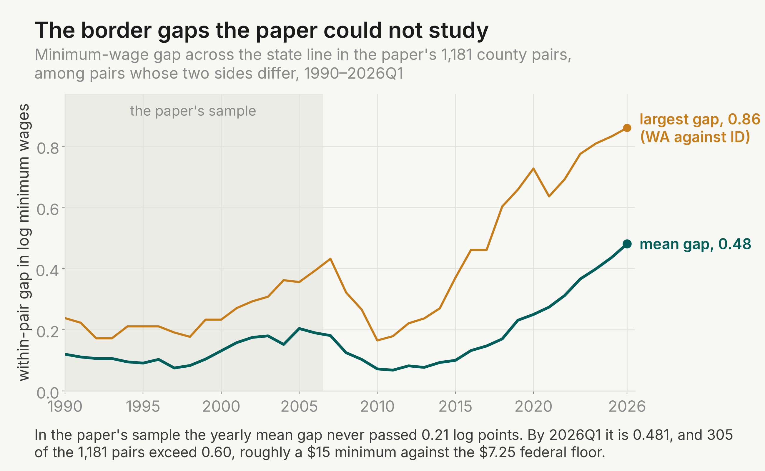
A reader asked, through the site, whether the no-job-loss finding holds now that cross-border minimum-wage differences are much larger. The paper raises this question itself. On page 962 the authors wrote that the results "cannot be extrapolated to predict the impact of a minimum wage increase that is much larger than what we have experienced". An estimate drawn from small minimum-wage differences need not predict what large ones do, because a larger minimum reaches further up the wage distribution. In the paper's balanced sample, the yearly mean gap among differing pairs stayed between 0.065 and 0.185 log points. Across all 1,181 pairs, as in Figure 2, it peaked at 0.204 in 2005.
The federal floor has been $7.25 since July 2009, while many states index or phase in much higher minimums. By 2026Q1, 828 of the paper's 1,181 pairs straddle a minimum-wage difference. Their mean gap is 0.481 log points. Of all 1,181 pairs, 305 exceed 0.60, roughly a $13.20 minimum against $7.25. The largest is 0.86: Washington's $17.13 against Idaho's $7.25.
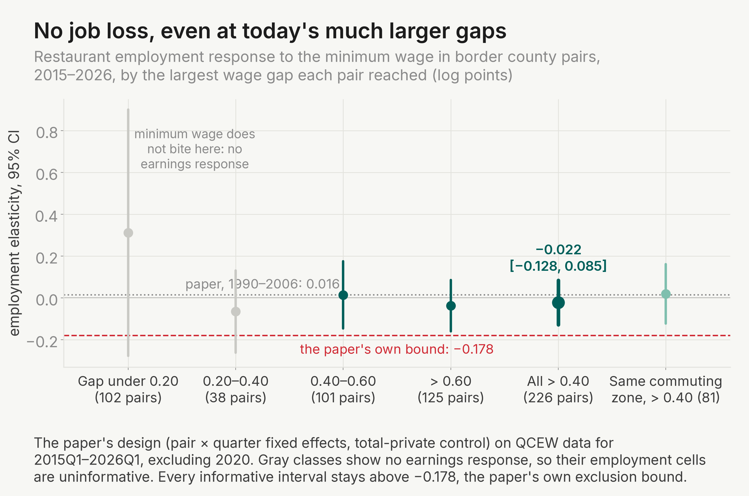
We extended the paper's QCEW restaurant panel from 2006 to 2026Q1. We grouped the 1,181 pairs by the largest gap each reached over 2015Q1 to 2026Q1, fixed before any employment outcome was examined. We then re-estimated the paper's preferred specification (pair-by-quarter fixed effects with the total private sector control) on 2015Q1 to 2026Q1, excluding 2020, within each class. Classes where the earnings response is not significant are uninformative: if the minimum cannot be shown to bite, a zero employment effect means nothing. That excludes the two classes with gaps under 0.40.
In the large-gap pairs, the answer matches the paper's. Across the 226 balanced pairs whose gap passed 0.40 (all 608 large-gap pairs average a 2026Q1 gap of 0.587 log points), the employment elasticity is −0.022 (s.e. 0.054). Its 95 percent confidence interval is [−0.128, 0.085]. The earnings elasticity is 0.121 (s.e. 0.015), so the minimum wage bites hard in these counties. The interval's lower bound, −0.128, lies above the −0.178 bound the paper itself ruled out. So the paper's conclusion extends, in the paper's own terms, to gaps two to four times larger than its average gap. The employment leads are tiny (−0.015 and −0.017, each less than a quarter of its standard error). So the higher-minimum counties were not already on different restaurant trends before the gaps opened.
| Gap class (largest gap reached, log points) | Balanced pairs | Employment (s.e.) [95% CI] | Earnings (s.e.) | Does it bite? |
|---|---|---|---|---|
| Under 0.20 | 102 | 0.312 (0.300) [−0.28, 0.90] | 0.220 (0.131) | not significant: uninformative |
| 0.20–0.40 | 38 | −0.065 (0.100) [−0.26, 0.13] | 0.094 (0.060) | not significant: uninformative |
| 0.40–0.60 | 101 | 0.015 (0.082) [−0.15, 0.18] | 0.128 (0.033) | yes |
| Over 0.60 | 125 | −0.037 (0.063) [−0.16, 0.09] | 0.118 (0.017) | yes |
| All over 0.40 | 226 | −0.022 (0.054) [−0.128, 0.085] | 0.121 (0.015) | yes |
Notes. All rows are our estimates; the paper has no counterpart at these gaps. The paper's preferred specification on QCEW data for 2015Q1–2026Q1 excluding 2020, with standard errors two-way clustered by state and border segment. A class bites when its earnings confidence interval excludes zero. The headline row's minimum detectable effect is 0.152, the size of loss this design would detect 80 percent of the time; the estimate itself rules out losses beyond −0.128.
A single regression that interacts the minimum wage with the gap classes asks the dose-response question formally. Does the employment effect grow more negative as the gap grows? No class differs significantly from another. The class slopes are 0.272, −0.049, −0.002 and −0.032 from the smallest class to the largest, and the test that all four slopes are equal gives p = 0.449. The contrast between the two classes over 0.40 and the two under it is −0.129 (s.e. 0.111). Between the two classes where the minimum bites, the difference is −0.030 (s.e. 0.058).
The result survives the variants we declared in advance:
- estimating only 2021Q1 to 2026Q1 gives 0.069 (s.e. 0.084);
- dropping 2021 as well as 2020 gives −0.014 (s.e. 0.058);
- dropping the California pairs once the state's $20 fast-food minimum takes effect gives −0.023 (s.e. 0.055);
- using all 608 large-gap pairs rather than the balanced 226 gives 0.002 (s.e. 0.056);
- adding a separate linear trend for every pair leaves the estimate at −0.022 (s.e. 0.039);
- dropping the total private sector control gives −0.047 (s.e. 0.054).
Every variant leaves the lower confidence bound above −0.178. The metro split is descriptive only, but all three groups are near zero: −0.029 (s.e. 0.050) for metro pairs, −0.036 (s.e. 0.108) for nonmetro, and −0.016 (s.e. 0.065) for mixed.
The longer panel also lets us re-run the paper's central diagnosis. The paper argues that designs without local controls read spatial heterogeneity as job loss. Its own years confirm that on our panel, which uses today's data vintage (see Notes): with common time effects the border sample gives −0.109 (s.e. 0.075), against −0.043 (s.e. 0.091) with the full pair-by-quarter effects. That wedge shrinks era by era and is gone today. On 2021 to 2026 the two specifications give 0.051 (s.e. 0.039) and 0.054 (s.e. 0.077), a difference of −0.003 (p = 0.95). As high minimums spread, the low-wage states that once trended differently stopped doing so. This is consistent with the paper's account of why the two designs disagreed.
Does the answer change when the minimum bites harder?
A gap across a border is not the same thing as a minimum that binds. Spokane County, Washington faces Idaho across the largest gap in the data, 0.86 log points. Yet Washington's $17.13 minimum is only 0.65 of the local median wage, because Washington wages are high. Today's large gaps come mostly from high-wage states bordering low-wage ones, so bindingness rises far less than the gap. Even Spokane, at the largest gap, only reaches the lower edge of the most binding tail, ratios of 0.65 and above; most large-gap pairs sit below it. The economic content is in bindingness. Competitive models predict that the employment response turns negative as the minimum rises toward the median wage. Search and monopsony models predict a response near zero up to some threshold.
Our second extension study writes the employment elasticity as a function of bindingness, the minimum divided by the local median wage. Area median wages start only in 2005, so the fit uses a mean-based stand-in that reaches back to 1990: 40 times the minimum, divided by the county's average weekly private-sector pay over the previous year. A line fitted on 2005 to 2026, where both measures exist, converts between them. The function itself is fitted on 1990 to 2014 only; the conversion line uses later years too. The fitted level at the sample's average bindingness is −0.026 (s.e. 0.079), and the slope is −0.007 (s.e. 0.011) per unit of the mean-based ratio: no detectable gradient. A kinked version places its best-fitting threshold at a median ratio of 0.62. But the kink's slope has a bootstrap 95 percent interval of [−25.63, 0.92], which spans zero. So no threshold is statistically identified over the data's range.
The pre-declared test holds the model out of sample: predict the 2015 to 2026 elasticity from the pre-2015 fit, then compare with the direct estimates. In the bins where today's large-gap pairs mostly fall, ratios of 0.45 to 0.65, the direct estimates of −0.019 and −0.021 land inside the prediction band. The tail at 0.65 and above is different. Only 4 pre-2015 pairs ever reached that bindingness, once their mean-based ratios are converted, so the pre-2015 data cannot discipline a prediction at the extreme tail of today's range. About 31 percent of today's large-gap pairs are in that tail. For that tail we claim nothing: the model's band there rests on only 4 pre-2015 pairs, so the effect is not yet tested, not zero.
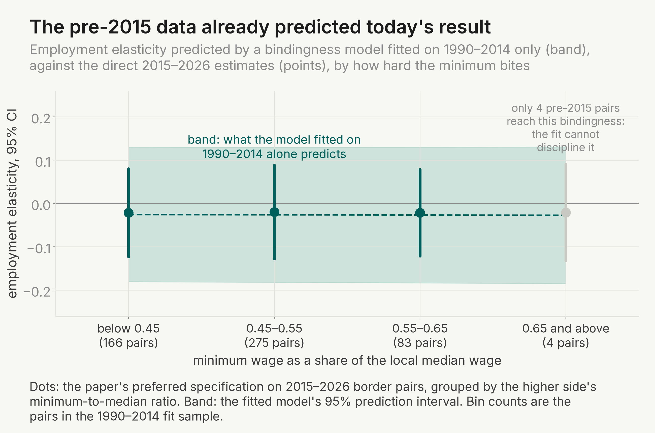
The model makes testable predictions, and they fall in that tail, so they will be its first real test. Washington against Idaho, Florida's $15.00 step against Alabama and Georgia, Michigan's $15.00 against Indiana and Ohio, and California's fast-food sector should all show employment elasticities near −0.03. A future estimate whose own confidence interval lies wholly below about −0.19 would falsify it. The implied own-wage employment elasticity (the paper's labor-demand elasticity) at the fit's center is −0.13 (s.e. 0.40). That is consistent with the median across published studies collected by Dube and Zipperer (2024, NBER working paper).
Does the commuting-zone critique change the answer?
Jha, Neumark and Rodriguez-Lopez (2024, NBER working paper) argue that many border pairs are poor comparisons. Two neighboring counties can still belong to different commuting zones, the areas within which most people both live and work. If they do, they are separate labor markets, and the authors argue this biases the border design toward zero. On County Business Patterns data for 1990–2016, their same-commuting-zone pairs give −0.160 (s.e. 0.107). On the paper's own 1990–2006 data, their commuting-zone pairs give −0.141 (s.e. 0.070), against 0.016 for all pairs.
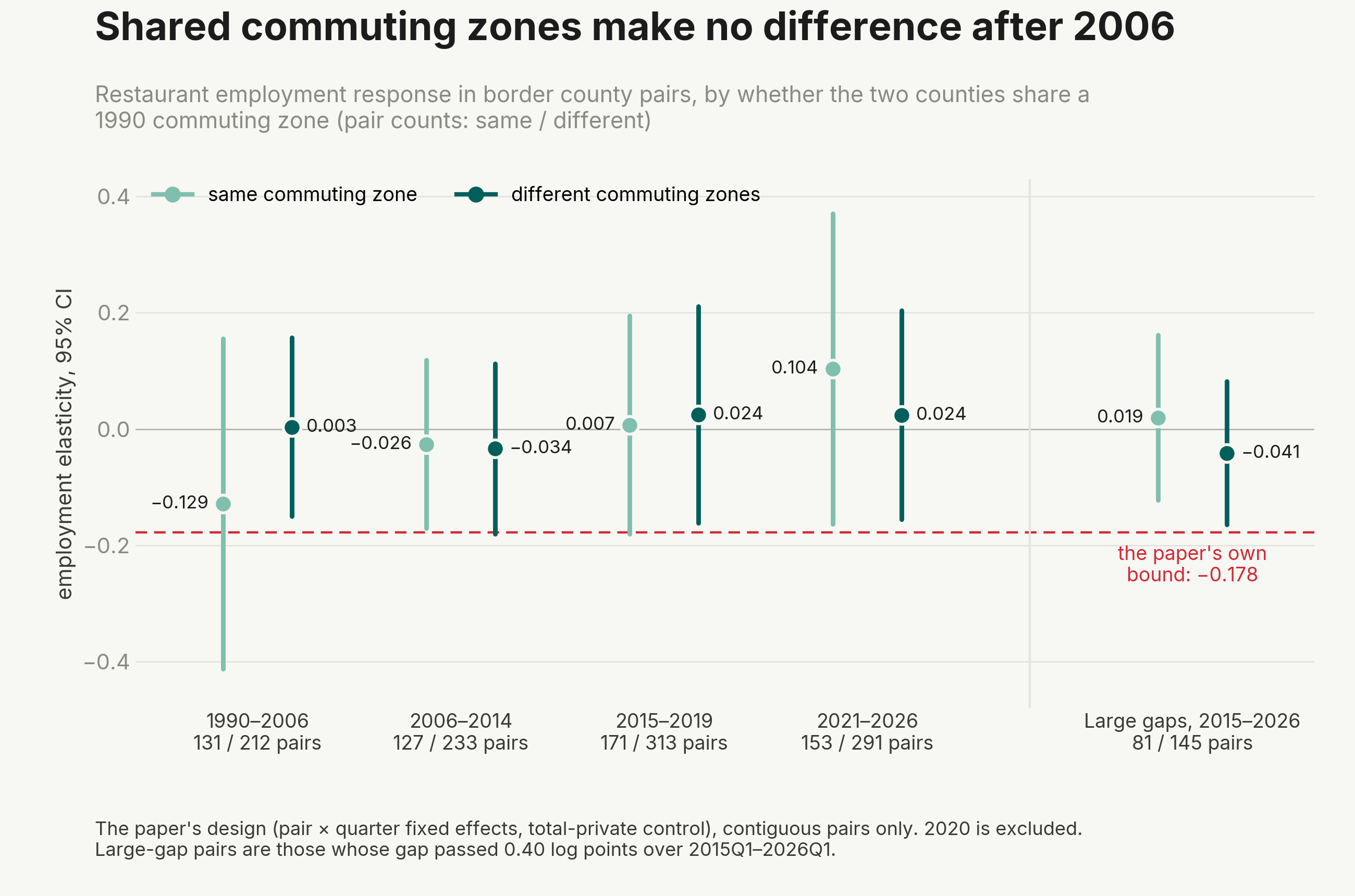
We split the paper's 1,181 pairs by whether both counties lie in the same 1990 commuting zone, the definition the critique uses. That gives 331 same-zone pairs. We then re-estimated the paper's preferred specification separately for the same-zone and different-zone pairs, era by era, and in the large-gap pairs.
| Years | Same zone: employment (s.e.) | Same zone: earnings (s.e.) | Different zones: employment (s.e.) | Different zones: earnings (s.e.) |
|---|---|---|---|---|
| 1990–2006 | −0.129 (0.145) | 0.211 (0.100) | 0.003 (0.078) | 0.170 (0.045) |
| 2006–2014 | −0.026 (0.074) | 0.097 (0.054) | −0.034 (0.075) | 0.157 (0.037) |
| 2015–2019 | 0.007 (0.096) | 0.176 (0.070) | 0.024 (0.095) | 0.183 (0.055) |
| 2021–2026 | 0.104 (0.136) | 0.144 (0.051) | 0.024 (0.092) | 0.126 (0.037) |
| Large-gap pairs, 2015–2026 | 0.019 (0.072) | 0.130 (0.028) | −0.041 (0.063) | 0.116 (0.019) |
Notes. All rows are our estimates. Balanced contiguous pairs, standard errors two-way clustered by state and border segment. The 2006–2014 era starts in 2006Q3, and 2020 is excluded throughout. Large-gap pairs are those whose gap passed 0.40 log points over 2015Q1 to 2026Q1 (81 same-zone and 145 different-zone pairs).
In the paper's years our same-zone estimate, −0.129 (s.e. 0.145), is close to the critique's. It rests on 131 pairs and the small gaps of that period, so its 95 percent interval, [−0.413, 0.155], is wide. After 2006 the two groups agree in every era. In the large-gap pairs the same-zone estimate is 0.019 (s.e. 0.072), against −0.041 (s.e. 0.063) for different-zone pairs. Earnings respond strongly in the same-zone large-gap pairs (0.130, s.e. 0.028), so the minimum bites there and the zero employment response is informative. One era is weaker: in 2006–2014 the same-zone earnings interval includes zero, so that era's same-zone employment estimate says little.
The answer does not depend on which commuting-zone map is used. With the 2020 commuting zones in place of the 1990 ones, the same-zone large-gap estimate is 0.071 (s.e. 0.087). One limit remains. The critique's broader samples also pair counties that share a commuting zone without touching. We ran touching pairs only, so this tests the critique on the paper's own pairs, not on its full sample.
Dube, Reich, Bhatt and Sosinskiy (forthcoming, Journal of Political Economy Microeconomics) reply to the critique with data that stop in 2019. That is before most of the large gaps opened, so neither side of the exchange had tested the large-gap era.
How this relates to later research
Taylor and West (2023, NBER working paper) run border pairs on limited-service restaurants and find urban losses (−0.040) against rural gains. Our metro and nonmetro large-gap splits are both near zero, though ours are descriptive and theirs are the paper's focus. Our metro estimate, −0.029 (s.e. 0.050), is close in size to their urban −0.040 (s.e. 0.013), but much less precise, and it covers all restaurants, not only limited-service ones. Our living page for Cengiz, Dube, Lindner and Zipperer (2019) reaches a similar conclusion through 2024 from different identifying variation. That design counts jobs missing below a new minimum against jobs appearing just above it, rather than comparing neighbors across a state line. The extension does not test hours, worker composition, prices or profits, and it keeps the paper's restaurant focus. A zero employment elasticity is compatible with adjustment on any of those margins.
Notes
These are the judgment calls and data limits behind our numbers, so you can decide how much weight each result deserves.
Show all 15 notes
- Stata is licence-gated in our container, so the whole replication is an R port of the authors' do-files. The cell-for-cell match on the main table is our evidence the port is faithful. A naive port gave standard errors off by about 35 percent until Stata's undocumented conventions were reconstructed.
- State minimum wages for 2008 to 2022 were rebuilt from the Department of Labor's annual history table. Mid-year increases in those years are therefore timed to the year, not the quarter. The 2023 to 2026 rates use effective-dated records. The gap classes are set by the largest gap reached, which the 2026 values dominate, and ten county spot-checks of the 2026Q1 panel all match official rates.
- For the same reason, a 2020-only estimate is unavailable here: the rebuilt series has no variation within 2020, although real mid-2020 increases (Nevada, Oregon, DC, Chicago, Cook County) did occur. The pandemic year is excluded from every estimate by design, and dropping 2021 as well changes nothing.
- Local ordinances before 2023 are coded at the state rate, which understates the minimum in cities such as Seattle, San Francisco and Chicago over 2015 to 2022. The Chicago, Cook County and Montgomery County ordinance rates before July 2025, and Flagstaff's before 2026, are also absent, so those county-quarters carry the state rate. The headline is insulated: its pairs differ state against state, and coding counties by population weight, by majority, or by state rate alone gives the identical −0.022. The codings differ only where a local ordinance is coded, and pre-2023 ordinances are absent from all three, so this is a limited test of the missing ordinances.
- The large gaps grew through slow, scheduled divergence that aligns with state politics. That is where a border design is weakest: pair-by-quarter effects absorb shared shocks but not trends that differ across the line. We pre-declared six mitigations, all reported above:
- the 2020 exclusion, with a drop-2021 variant;
- employment leads by era;
- the same-commuting-zone cut;
- pair-specific linear trends;
- an earnings response check per class;
- claiming an extension only when the confidence interval clears the paper's own −0.178 bound.
- The pair-trend variant leaves the point estimate unchanged by construction, since pair-by-quarter effects already absorb trends the two counties share. Its smaller standard error, 0.039, comes from a different clustering formula, not added precision. The employment leads are imprecise (s.e. 0.061 and 0.084), so they bound pre-trends only loosely.
- The headline uses pairs with complete data over the estimation window, 226 of the 608 large-gap pairs; the unbalanced variant is 0.002 (s.e. 0.056).
- The minimum raises restaurant earnings less per log point today than in the paper's years, 0.121 against 0.188. So the same −0.178 bound allows somewhat more job loss per unit of pay gained.
- The largest gap any pair reached in the paper's years was 0.393, in 2006, so every pair in the headline class went past it.
- Connecticut replaced its counties with planning regions in the 2024 data, so its 14 pairs are dropped from 2024Q1. Their gaps are all 0.122 or less, so no large-gap variation is lost.
- Retail, which employs 16.4 percent of near-minimum workers according to the paper, is near zero in every era: a second low-wage sector without detectable job loss. Manufacturing shows −0.07 to −0.13, none significant (s.e. 0.095 to 0.134). A negative value means the higher-minimum side lost manufacturing relative to its neighbor, which fits trends that differ across the line.
- The bindingness measure matches a county to its official wage-area median for 73.9 percent of county-quarters overall. In the recent years that drive the test the match rate is 94 to 100 percent. Unmatched county-quarters are dropped, never imputed.
- The bindingness estimates residualize on county once and then absorb pair-by-quarter effects. That is exact for the headline estimate, but only approximate for the bindingness terms, because many counties belong to more than one pair. Read the gradient, the bin estimates and the predictions as approximate. The four named predictions, like Spokane, sit at ratios of 0.65 and above, where the pre-2015 data give the model little support.
- On our rebuilt panel the paper-era anchor is −0.043 (s.e. 0.091) against the paper's 0.016. Most of the difference is sample composition: the current data vintage suppresses more cells. On the package's own sample our current-vintage estimate is −0.007, so the rest comes from data revisions.
- The commuting-zone check uses touching pairs only. The authors' broader samples, which add non-touching pairs in the same zone, are not run here.
Data sources for the extension studies
The extension studies pulled fresh public data on October 14, 2026. In full:
Show all 7 sources
- U.S. Bureau of Labor Statistics, Quarterly Census of Employment and Wages: bulk quarterly-by-industry files 1990–2013 and open-data API quarterly slices 2014Q1–2026Q1 (county level; restaurants, retail, manufacturing and total private), current vintage as published; 2026Q1 released August 28, 2026.
- U.S. Bureau of Labor Statistics, Occupational Employment and Wage Statistics: all-occupation area wage medians for May 2005, 2010, 2015, 2019, 2022 and 2025, with the May 2024 and May 2025 area-definition files (the bindingness study).
- U.S. Department of Labor, Wage and Hour Division: the state minimum-wage history table (January 2025 version), used for annual state rates 2008–2022, and 12 dated versions of the consolidated state minimum-wage page (live and Internet Archive captures, 2022–2026), compiled into an effective-dated 2023–2026 change file.
- New York Department of Labor and Oregon Bureau of Labor and Industries regional tier schedules (Oregon's nonurban county list from ORS 653.026), and the official minimum-wage pages of Chicago, Cook County IL, Montgomery County MD, Las Cruces NM and Flagstaff AZ for border-county local ordinances.
- U.S. Census Bureau county population estimates: 1990 intercensal, 2000–2010 intercensal, Vintage 2020 (2010–2019) and Vintage 2025 (2020–2025), plus the Vintage 2025 subcounty file for the population weights of city ordinances.
- David Dorn's county-to-commuting-zone crosswalk (Tolbert–Sizer 1990 zones, ddorn.net) and the USDA Economic Research Service 2020 commuting-zone delineation.
- Dube, Lester and Reich's replication data and code, Harvard Dataverse doi:10.7910/DVN/L4DUZ7, version 2.0 (CC0): the QCEW extracts, the pair list and the pre-2008 minimum-wage series, reused for the replication, the anchor checks and the 1990–2007 panel years.
The bindingness study fetched no data beyond the wage medians above; it works from the living update's panel. No CPS or other microdata enter either study, and all elasticities compare within pair and quarter, so no price deflator is used.
The full replication working directory, including both extension studies, is public at github.com/living-sciences/living-minimum-wage-borders.
Discussion
Sign in to join the discussion.
Loading discussion…