Raising taxes by 1 percent of GDP lowers real GDP by about 3 percent over the following ten quarters. Romer and Romer (2010) found this for the postwar decades, and it still holds with data through 2026.
The difficulty is that many tax changes respond to the economy. Congress cuts taxes to fight slowdowns and raises them to pay for new spending, so a simple regression of output on tax changes is biased. Romer and Romer read the record behind every federal tax bill from 1945 to 2007. They keep only the changes passed for reasons unrelated to current conditions, such as reducing an inherited deficit or raising long-run growth. These exogenous tax changes are the paper's measure of tax shocks.
What we found:
- The paper's results reproduce from the authors' data. Our rewrite of their analysis gives the printed headline, a peak fall of 3.08 percent.
- The 3 percent holds through 2026. With tax changes coded by later researchers, the peak fall through 2019 is 2.93 percent, the paper's own number. Through 2026:Q3, with recent acts we coded ourselves and the pandemic quarters left out, it is 2.91 percent (t up to −3.10).
- Two secondary claims are weaker than the paper states. The paper finds that output responds when a tax change takes effect, not when it is announced, but that rests on the Korean War years 1950 to 1952. Without them, announcements appear to matter too. The paper also argues that simpler measures of tax changes understate the effect. Once the early years are set aside, that holds for one measure, cyclically adjusted revenues, but not for the sum of all legislated tax changes.
The paper's main claims
- A tax increase of 1 percent of GDP lowers real GDP by 3.08 percent (t = −3.53) ten quarters later. This is the peak, the largest fall in any quarter after the change. It comes from regressing output growth on twelve quarterly lags of the exogenous series over 1950:I–2007:IV. Adding past output growth as a control gives −3.02 (t = −2.90). A two-variable vector autoregression (VAR), in which output and the tax series can affect each other, gives −2.93 (t = −2.80).
- The series behaves like a random shock. Its mean is −0.03 percent of GDP, its standard deviation is 0.24, and it is not correlated with its own past. Past output growth does not predict it (Granger causality p = 0.78).
- Broader measures of tax changes give much smaller effects. The change in cyclically adjusted revenues gives a peak of −1.10 (t = −2.27), or −1.21 (t = −2.08) in a VAR. The sum of all legislated changes, whatever their motive, gives −1.86 (t = −2.74). The paper attributes the gap to omitted-variable bias: the broader measures include changes that respond to the economy.
- Output responds when a tax change takes effect, not when it is announced. The series of changes taking effect gives a peak of −3.50 (t = −2.22). The present value of changes already legislated but not yet in force has a coefficient of +1.10 (t = 1.17). The paper concludes that anticipation effects are of secondary importance.
- The response is smaller after 1980: a peak of −4.29 before 1981 against −3.08 after.
- Investment drives the fall. Gross private domestic investment falls 11.19 percent (t = −3.35) and consumption 2.55 percent (t = −3.06). Imports fall 10.07 percent (t = −3.62), and exports rise 4.98 percent (t = 2.08).
- The two kinds of exogenous change give different results. Changes made for long-run reasons alone give −2.99 (t = −2.92). Changes made to reduce an inherited deficit give +2.48, but with t = 1.03 the paper calls that estimate too imprecise to interpret.
What we were able to do
The authors posted their data in one spreadsheet, Romer&RomerFiscalData.xlsx (115 KB). It holds the quarterly tax series, its present-value version, the series split by motive, and output data as measured in 2008. Their estimation programs are written in RATS, a commercial package we do not have, so we rewrote the analysis in Python. The single-equation regressions use least squares. For everything the paper estimates by VAR, we use the same Monte Carlo method with 10,000 draws and three random seeds. One detail appears only in the programs, not in the paper: each regression takes its lagged values from the quarters before the sample starts. So the 1950:I–2007:IV regressions draw their lags from 1947–1949. We checked every output of our rewrite against the paper's printed tables and figures.
For the extension, we used the national accounts as published by the BEA in 2026 (1947:Q1–2026:Q3). For 2008–2019 we used tax changes that later researchers coded the paper's way, from three sources:
- Liu and Williams (2019) carried the narrative coding past 2007, act by act;
- Mertens (2018) coded the Tax Cuts and Jobs Act;
- Cloyne, Martinez, Mumtaz and Surico (2025) collect both into a series ending 2019:Q4.
Together they add three nonzero quarters:
- the 2010 extension of the Bush tax cuts, −0.44 percent of GDP at 2011:Q1;
- the American Taxpayer Relief Act, −0.41 at 2013:Q1;
- the Tax Cuts and Jobs Act, −1.00 at 2018:Q1.
No published coding covers 2020–2026, so we coded those acts ourselves, using the paper's categories. We wrote down the coding before estimating anything. For the pandemic acts and the Inflation Reduction Act, our dollar figures come from public documents that report the Joint Committee on Taxation's (JCT) revenue estimates. For the 2025 act they come from JCT's own tables, which estimate the revenue effect of each provision. We also used the monthly federal funds rate, for the analysis of monetary policy below.
What we got when we re-ran it
Our rewrite reproduces the headline exactly, once we use the paper's convention for lags. Our single-equation peak is −3.08 (t = −3.53), the printed value, and the VAR gives −2.95 against the printed −2.93. The tax series has the properties the paper states: mean −0.03, standard deviation 0.24, Granger p = 0.78. The robustness checks hold too. Dropping the largest acts one at a time keeps the peak between −2.23 and −3.42, against the paper's −2.20 to −3.39.
The headline and its variants (published / this re-run)
| Specification | Published | Ours |
|---|---|---|
| Single equation (eq. 6) | −3.08 (t = −3.53) | −3.08 (t = −3.53) |
| With lagged output growth (eq. 7) | −3.02 (t = −2.90) | −3.03 |
| Two-variable VAR | −2.93 (t = −2.80) | −2.95 (t = −2.79) |
| Implementation series (eq. 8) | −3.50 (t = −2.22) | −3.50 (t = −2.22) |
| News (present-value) series (eq. 8) | +1.10 (t = 1.17) | +1.10 |
| Long-run changes only | −2.99 (t = −2.92) | −3.00 (t = −2.91) |
| Deficit-driven changes only | +2.48 (t = 1.03) | +2.46 |
| 1950–1980:IV | −4.29 | −4.26 (t = −2.19) |
| 1981–2007:IV | −3.08 | −3.08 (t = −3.35) |
| From 1955 (post-Korea) | −2.63 (t = −2.68) | −2.56 (t = −2.60) |
Notes. Each cell is the peak cumulative response of real GDP, in percent, to an exogenous tax increase of 1 percent of GDP. The sample is 1950:I–2007:IV unless the row names another. VAR cells are means over 10,000 Monte Carlo draws per seed, three seeds; the seed spread is at most 0.05. Our deficit-driven cell is a point estimate without a Monte Carlo t. Italicised cells are ours.
The paper also concludes that output responds to a tax change when it takes effect, not when it is announced. That conclusion depends on the first three years of the sample, 1950 to 1952. The paper tests it (its equation 8) by putting two series in the same regression. The implementation series records the tax changes taking effect in each quarter. The news series records the present value of changes already legislated but not yet in force. A positive news coefficient means output rises while a tax increase is pending, as it would if people moved work and spending ahead of the increase. On the full sample the news coefficient is +1.10 (t = 1.17) and the implementation coefficient is −3.50, so the paper reads anticipation effects as secondary.
Starting the sample in 1953:I instead of 1950:I pushes both coefficients further from zero. The implementation coefficient grows to −4.34 (t = −3.24) at its peak, seven quarters after the change; on the full sample the peak comes at ten. The news coefficient more than doubles, to +2.37 (t = 1.7). So once the first three years are dropped, the paper's evidence that announcements matter little is gone. With a t-statistic that low, though, the data do not clearly show that they matter either.
The headline single-equation regression, which leaves out the news series, moves the other way. On the same 1953:I start its peak shrinks from −3.08 to −2.65 (t = −3.39), reached at eight quarters instead of ten. So the headline holds up without those three years, at 14 percent smaller.
The first three years matter because they contain the Korean War boom. The boom came within ten quarters of the 1948 tax cut, the largest entry in the series (−1.87 percent of GDP). So it falls inside the period over which the regression measures that cut's effect. The war's own tax increases are excluded because they paid for spending, so nothing in the series explains the boom. The regressions therefore count part of the boom as a response to the 1948 cut. We treat the question of whether announcements matter as unresolved.
The paper's comparison with broader tax measures also reproduces, in direction. The broader measures are the change in cyclically adjusted revenues and the sum of all legislated changes, whatever their motive. Our cyclically adjusted revenue effects are about 13 percent larger than printed: −1.24 against −1.10 in the single equation, and −1.37 against −1.21 in the VAR.
We also ran a test the paper does not report. Before 1960 the cyclically adjusted revenue series is not measured; it is backcast from output growth. So in the earliest years this tax measure is partly built from the output it is supposed to explain. Part of the full-sample gap therefore comes from how the series is built. The cleaner comparison starts in 1955, after the Korean War, though five backcast years remain. On that sample our exogenous series gives −2.56 (t = −2.60) against the paper's −2.63.
From 1955 the two broader measures behave differently. All legislated changes together give −2.48, against the paper's −2.36. That is within 0.2 of the exogenous estimate. Computed inside each Monte Carlo draw, the difference between the two has t = −0.48, so for this measure the gap closes, as the paper concedes. Cyclically adjusted revenues give −1.55, matching the paper's −1.57. Here a gap of about 1 point remains: the difference computed the same way is −1.04, with t = −1.91. So the claim that broader measures understate the effect survives for cyclically adjusted revenues, the standard measure, though the difference falls short of significance. It does not survive for the sum of all legislated changes. The gap is also smaller than on the full sample. From 1955 on, the cyclically adjusted estimate is 40 percent below the exogenous one, against 64 percent below on the full sample.
The paper's Table 1 adds one control at a time to the VAR, to check whether something that moves with taxes explains the result. These checks reproduce. Our peaks for the six rows are within 1.5 percent of the printed values, and the estimate stays significant under every control. One standard error differs: for the row adding the Romer and Romer monetary shock, ours is 1.46 against the printed 0.90. We could not trace the gap.
The paper's Table 1: adding a control to the VAR (published / this re-run, peak response with standard error)
| Added control (sample) | Published | Ours |
|---|---|---|
| Government spending (1950–2007) | −2.75 (1.07) | −2.75 (1.09) |
| Relative price of oil (1950–2007) | −2.54 (1.07) | −2.55 (1.06) |
| Romer and Romer monetary dummy (1950–2007) | −2.32 (0.96) | −2.31 (0.95) |
| Federal funds rate (1953–2007) | −2.18 (0.80) | −2.16 (0.81) |
| Romer and Romer monetary shock (1972–1996) | −3.61 (0.90) | −3.66 (1.46) |
| Republican president dummy (1950–2007) | −3.07 (1.00) | −3.07 (1.01) |
Notes. Each cell is the peak response of real GDP, in percent, to a tax increase of 1 percent of GDP in a three-variable VAR with the named control. Standard errors are in parentheses. Our standard errors are implied by each estimate's Monte Carlo t. Italicised cells are ours.
The components of GDP (published / this re-run, peak response in percent)
| Published | Ours | |
|---|---|---|
| Consumption | −2.55 | −2.54 |
| Gross private domestic investment | −11.19 | −11.18 |
| Durables | −8.27 | −8.25 |
| Nondurables | −2.27 | −2.27 |
| Services | −1.30 | −1.41 |
| Nonresidential fixed investment | −8.50 | −8.48 |
| Residential fixed investment | −5.84 | −5.79 |
| Exports | +4.98 | +0.06 |
| Imports | −10.07 | −10.03 |
Notes. Three-variable VARs with the shock, GDP and the named component, on the full 1950:I–2007:IV sample. Services peaks at twelve quarters in our run against the paper's eight. The exports row is the one failure: our response is flat where the paper's rises 4.98 percent (t = 2.08). We have no explanation for it. Everything else is within 0.11 of the printed value.
The same analysis on today's data
The paper's data end in 2007, so the obvious question is whether the last two decades change the answer. Revisions to the old data do not. On the paper's own sample, the 2026 version of the output data moves the VAR peak from −2.95 to −2.99, and growth rates in the two versions correlate at 0.991. So the results below reflect the new years, not new measurements of the old ones.
Through 2019, on published shocks
Adding 2008–2019, with the three published tax changes, gives a VAR peak of −2.93 (t = −2.98) at ten quarters. That is the number the paper prints for 1950–2007. Splitting by motive gives the same picture as before: long-run changes give −3.05, deficit-driven changes +2.49. The 2017 Tax Cuts and Jobs Act can also be valued another way. Counting its one-time international provisions as offsetting revenue makes its net cost $135 billion a year instead of $204 billion. Its shock then becomes −0.66 percent of GDP instead of −1.00, and the peak is −3.01 (t = −2.99). Either way, the paper's headline describes 1950–2019 as well as it described 1950–2007.
To 2026, with acts we coded ourselves
For 2020–2026 we coded the acts ourselves. The pandemic acts of 2020–2021 (CARES, the Families First act and the American Rescue Plan) were passed to fight the downturn. The paper's method excludes such changes, because they respond to the economy, so these acts add nothing to the series. The Inflation Reduction Act of 2022 raised revenue to narrow the deficit, through a corporate minimum tax and a tax on stock buybacks. It enters as +0.10 percent of GDP at 2023:Q1.
The One Big Beautiful Bill Act of 2025 is harder to code, because it does two things. Most of its revenue cost comes from continuing the 2017 act's rates, which were scheduled to expire at the end of 2025. The paper's rules do not count a law that merely extends an existing tax. The rest of the act is new, and much of it applies from 2025. It includes:
- full expensing of equipment and of domestic research spending;
- a higher cap on the deduction for state and local taxes;
- deductions for tips, overtime and seniors.
So we coded the act both ways, using JCT's tables and recording each provision in the quarter it changes what taxpayers owe.
Counting only the new provisions gives a cut of 0.65 percent of GDP at 2025:Q3. Two small increases follow. The first, +0.04 at 2025:Q4, comes from ending the clean vehicle credits. The second, +0.14 at 2026:Q1, is the net of the provisions starting in 2026: the end of several clean energy credits and changes to opportunity zones outweigh the new cuts. Counting the continuation as well, as a cut relative to the scheduled expiration, turns the 2026:Q1 entry into −1.14. That is larger than the 2017 act's −1.00. It is smaller than the two largest entries since the 1948 cut: −1.36 for the 1982 Reagan installment and −1.28 for the 1964 Kennedy-Johnson cut.
The pandemic creates a problem for the estimation. Output fell 8.2 percent in 2020:Q2, for reasons that have nothing to do with taxes. That quarter came nine quarters after the 2017 act took effect in 2018:Q1, and the rebound came ten quarters after. Those are exactly the horizons where the response peaks. So if the pandemic quarters stay in, the regression reads the collapse and rebound as part of the response to the 2017 act, the one large recent shock. With no adjustment, the 1950–2026:Q3 VAR peak is −2.53 to −2.66, depending on the coding of the 2025 act. The drop from −2.93 comes from those quarters, not from the taxes.
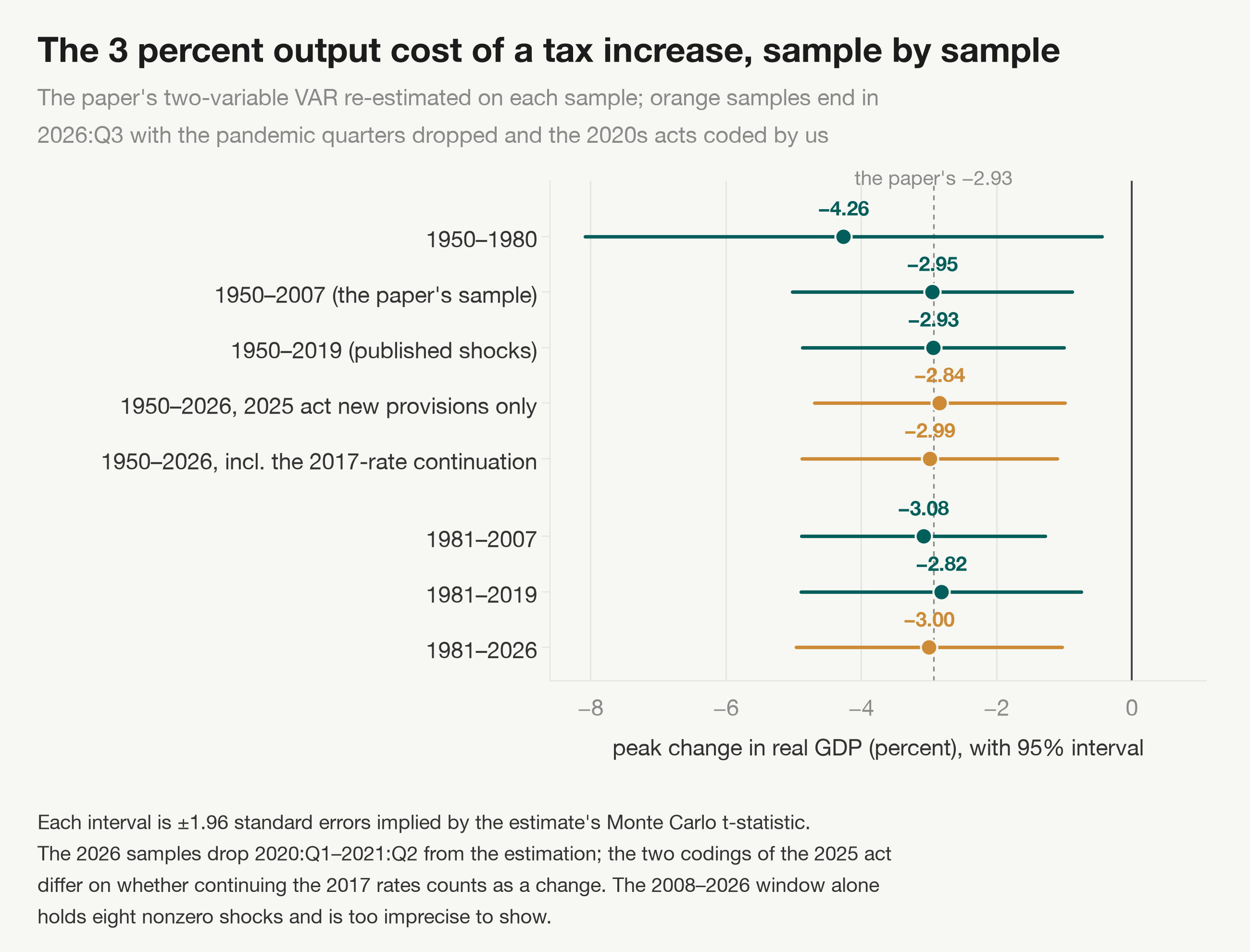
The standard fix, following Lenza and Primiceri (2022, Journal of Applied Econometrics), is to drop the six quarters 2020:Q1–2021:Q2 from the estimation. That gives −2.84 (t = −3.01) when only the 2025 act's new provisions are counted, and −2.99 (t = −3.10) when the continuation is counted too. The midpoint is −2.91, indistinguishable from the −2.93 through 2019. The two codings differ by 5 percent of the estimate, so the answer does not depend on how that act is counted.
The narrow reading: carried to 2026:Q3 with the pandemic quarters set aside, the effect is −2.9, the paper's number. The added years do not detectably change the headline.
Has the effect weakened over time?
The paper describes this two ways. Its introduction calls the post-1980 response substantially smaller, while its Section VI.B calls the evidence of change modest. The longer sample supports the modest reading. The peak is −4.26 (t = −2.19) on 1950–1980 and −3.08 (t = −3.35) on 1981–2007. The paper itself prints −3.08 for both the full sample and the post-1980 one.
Adding recent years keeps the post-1980 estimate near 3 percent. On 1981–2019 the peak is −2.82 (t = −2.67). On 1981–2026, with the pandemic quarters dropped, it is −3.00 (t = −2.99), or −2.70 counting only the 2025 act's new provisions. The years after 2007 cannot answer the question on their own. The 2008–2026 window holds only eight nonzero shock quarters, and its estimate of −2.15 (t = −0.80) is too imprecise to interpret. So only the early window, before 1981, gives a large estimate. Every window since 1981 that is precise enough to read gives an effect near 3 percent.
How the funds rate responds to the shocks
Why is the 1950–1980 estimate larger? The paper's Figure 13B points to monetary policy. In that figure, after 1980 the Federal Reserve tends to lower interest rates after a tax increase; before 1980 the response moves up and down and is never significant.
We re-estimated that response in a VAR with three variables: the tax series, the federal funds rate and GDP. On 1981–2007, a tax increase of 1 percent of GDP is followed by a fall in the funds rate that reaches 1.29 percentage points after eight quarters. That easing would offset part of the contraction. On 1950–1980 the funds rate first rises, by up to 1.04 points in the first year. It then falls by at most 0.92 points, nine quarters after the change.
So before 1980 there is less easing to offset the tax increase, and it comes after a tightening. This lines up with the output estimates: the period with less easing is the one with the larger fall in output. But this compares only two periods, so it describes the pattern rather than testing the mechanism.
How this relates to later research
The paper's tax series became a standard input for later work, including the studies our extension builds on:
- Mertens and Ravn (2013, American Economic Review) use the shocks as instruments in a structural VAR, rather than regressing output on them directly. They also separate personal from corporate income tax changes. They measure effects per percentage point of the average tax rate, not per percent of GDP. They find that cutting the average personal income tax rate by 1 percentage point raises GDP by about 1.4 percent on impact. Because the two papers measure different experiments, their numbers do not convert one for one.
- Cloyne (2013, American Economic Review) builds the same kind of narrative series for the United Kingdom. He finds that a tax cut of 1 percent of GDP raises output by about 2.5 percent over three years, close to the paper's magnitude.
- Cloyne, Martinez, Mumtaz and Surico (2025, NBER Working Paper 30246) extend the series to 2019. They find that personal tax cuts raise output only briefly, while corporate tax cuts raise R&D and productivity for eight to ten years.
Our extension does not test these claims about personal and corporate taxes, because it keeps the paper's single combined series. It also does not test anticipation effects after 2007.
Notes
These are the judgment calls and data limits behind our numbers, so you can decide how much weight each result deserves.
Show all 9 notes
- The 2020–2026 acts are coded by us, not by the authors. We followed the paper's motive categories, using the statutes and public summaries. For the pandemic acts and the Inflation Reduction Act, the revenue figures are secondhand, from CRS and other summaries of JCT's estimates. The 2025 act is coded from JCT's own tables, which estimate every provision twice: once assuming the 2017 rates would have continued anyway, and once assuming they would have expired. The difference between the two is the continuation, which is why the page reports the act under both codings. The 2026 headline moves by about 5 percent between them.
- JCT reports revenue by fiscal year, so we had to choose which year's figure to use as each provision's annual effect. We use fiscal 2027. It is the first year in which every provision effective in 2025 or 2026 is in force for all twelve months, and it contains no one-time refunds for earlier years. We divide by fiscal 2027 GDP, projected one year ahead at the latest year's growth rate. Using fiscal 2026 instead gives −2.84 and −2.94 for the 2026 headline. Provisions effective in July 2026 add +0.002 percent of GDP at 2026:Q3. Provisions effective later fall outside the sample.
- The 2026 headline drops the six quarters 2020:Q1–2021:Q2 from the estimation. Keeping them gives −2.53 to −2.66, depending on how the 2025 act is coded. Another common fix adds a separate indicator for each of those quarters to every equation. This gives the same point estimates as dropping those quarters, because each indicator fits its quarter exactly.
- We could not extend the test of anticipation effects. The paper's series of legislated future changes ends in 2007:Q4, and no published source continues it. So our 2019 and 2026 estimates date each tax change only by when it took effect. This matters for the two largest recent acts. The 2017 act was passed in 2017:Q4 and took effect in 2018:Q1. The 2025 act was passed in July and made retroactive to the start of the tax year. Any effect of their announcement is missed.
- We coded the Inflation Reduction Act as exogenous because its revenue provisions were passed to narrow the deficit. The act also funds climate and health spending, so it could instead be classed with the spending-driven changes, which the method excludes. Excluding it moves the 1950–2026 estimate from −2.66 to −2.68 before the pandemic quarters are dropped.
- Every headline number is the largest response across horizons, picked from the estimated response at each horizon. The uncertainty is large: the 95 percent band around the paper's −2.93 runs from about −0.9 to −5.0. A tax change of 1 percent of GDP is also large for this series. It equals 4.2 standard deviations, and most changes in the series are small.
- VAR estimates are Monte Carlo averages over three seeds of 10,000 draws each. Across seeds they differ by at most 0.02 on the headline rows. Figure 1's intervals are ±1.96 standard errors implied by each estimate's Monte Carlo t.
- The funds rate series begins in July 1954. In the funds-rate VAR, earlier quarters are filled with its first observed value, so the 1950–1980 response effectively comes from the quarters after mid-1954.
- Our exports response (+0.06) does not match the paper's (+4.98), and we could not find out why. It does not affect the headline, which uses GDP alone.
Data sources for the extension studies
The extension studies pulled fresh public data on November 9, 10 and 14, 2026. In full:
Show all 7 sources
- Bureau of Economic Analysis, NIPA Tables 1.1.3 (real quantity indexes, GDP and components) and 1.1.5 (nominal GDP), 2026 vintage, 1947:Q1–2026:Q3, via the dbnomics API (accessed November 9, 2026).
- Liu and Williams (2019), "State-level implications of federal tax policies", Journal of Monetary Economics 105: 74–90, doi:10.1016/j.jmoneco.2019.04.005; the act-by-act record as reproduced in Chang Liu's 2020 University of Wisconsin–Madison dissertation, pp. 124–126 (accessed November 9, 2026).
- Mertens (2018), "The near term growth impact of the Tax Cuts and Jobs Act", Federal Reserve Bank of Dallas Working Paper 1803, Table 1.
- Cloyne, Martinez, Mumtaz and Surico (2025), "Short-Term Tax Cuts, Long-Term Stimulus", NBER Working Paper 30246, October 2025 revision, Appendix B (the published shock series to 2019:Q4).
- Hand-coded 2020–2026 revenue figures, accessed November 9–14, 2026: CRS Report R46279 (CARES Act, JCT estimate of −$543.4 billion over ten years); JCT JCX-13-21 as reported by Law360 (American Rescue Plan, about −$593 billion); JCT estimates as reported by Gibson Dunn (Inflation Reduction Act, +$296 billion over ten years); JCT, JCX-34-25 and JCX-35-25 (July 1, 2025), estimated revenue effects of the tax provisions of H.R. 1 as passed by the Senate and enacted unchanged, relative to the current-policy and present-law baselines (One Big Beautiful Bill Act; accessed November 14, 2026).
- Federal Reserve Board H.15, effective federal funds rate, monthly, July 1954 to October 2026, via dbnomics.
- Romer and Romer (2010), American Economic Review 100(3): 763–801, doi:10.1257/aer.100.3.763, with the data deposit
Romer&RomerFiscalData.xlsx, reused unchanged for every quarter through 2007.
The full replication working directory, including the extension studies, is public at github.com/living-sciences/living-tax-shocks.
Discussion
Sign in to join the discussion.
Loading discussion…